Part 1 — What Is Fine-Tuning? Teach an Existing Model a New Job

Download the matching self-contained notebook · Read the notebook preview

What you will build

Fine-tuning starts from learned numbers and adjusts them using examples. Before looking at a large model, we will make that change visible with one weight: prediction = w × x. The existing weight is 2, the input is 2, and the desired answer is 6.

A single small gradient step moves the prediction closer to 6. This miniature example gives us names for the quantities we will reuse: parameter, prediction, target, loss, gradient, and learning rate.

By the end: Measure one weight update by hand and verify it with PyTorch.

What you need before starting

You need basic Python: variables, functions, dictionaries, loops, and imports. When this lesson introduces a class or a library-specific term, its role is explained below.

Use Python 3.12. These examples were executed on Windows with Python 3.12.4. Use the shown interpreter consistently when installing packages and running code. This is an original small CPU teaching experiment, not a downloaded general-purpose LLM.

You do not need to run an earlier article to make this part execute. The complete files and data used here are supplied below. The series order is for learning the ideas progressively.

Understand the idea before the code

A model is a calculation with adjustable numbers. Feed it an input and it calculates an output. A parameter, also called a weight in this introductory example, is one of those adjustable numbers. A Python model class defines the calculation; the stored parameter values determine the particular model's behavior.

Training changes parameter values using examples. Pretraining is an earlier training stage that provides a starting model. Fine-tuning is further training from that starting point for a particular task. Inference is using the current parameters to make a prediction without updating them. These words describe different activities; calling a model for an answer does not automatically train it.

Our first model is prediction = w * x. x is the input, w is the adjustable weight, and target is the answer we want for that training example. A loss is a mismatch score: smaller is better according to the chosen formula. An optimizer is the algorithm that changes weights to try to lower that loss.

A gradient says how sensitive the loss is to a weight and in which direction a small weight change increases it. In the one-weight example it is a single number. We subtract a small multiple of it to move toward lower loss. The learning rate is that step-size multiplier; it is not a percentage improvement.

A picture of this part's idea

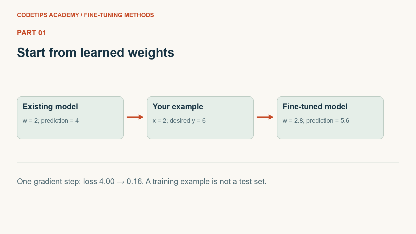
This picture introduces the mechanism. The numbers and assertions in the program below are the actual experiment.

Create the lesson folder

Create this folder and keep the filenames exactly as shown. In particular, a local module is an ordinary file beside the program, not an extra package you must guess how to install.

lesson-folder/
  lesson.py
  requirements.txt

Save requirements.txt

These are the external Python packages for this lesson. The local files above are included in the article; they are not pip packages.

torch==2.2.2
numpy==1.26.4
matplotlib==3.9.1

python -m venv .venv
.venv\Scripts\python.exe -m pip install -r requirements.txt

On Linux/macOS, use python3 -m venv .venv and .venv/bin/python -m pip install -r requirements.txt. Installation requires internet access. The default examples do not call a paid API.

Complete code for this article

Save this complete file as lesson.py

This is the complete program, including imports, data, function definitions, and the entry point.

def main():
    import torch

    w = torch.tensor(2.0, requires_grad=True)
    x, target = (torch.tensor(2.0), torch.tensor(6.0))
    loss = (w * x - target) ** 2
    loss.backward()
    print("before:", w.item(), "loss:", loss.item(), "gradient:", w.grad.item())
    with torch.no_grad():
        w -= 0.1 * w.grad
    new_loss = (w * x - target) ** 2
    print("after:", w.item(), "prediction:", (w * x).item(), "loss:", new_loss.item())
    assert abs(w.item() - 2.8) < 1e-05
    assert new_loss < loss


if __name__ == "__main__":
    main()

Run it and compare the result

Run commands from the lesson folder. In the commands below, python means the environment you installed into. On Windows, substitute .venv\Scripts\python.exe; on Linux/macOS substitute .venv/bin/python. Do not create the environment with one interpreter and run the lesson with another.

Run 1: python lesson.py

python lesson.py

Captured standard output:

before: 2.0 loss: 4.0 gradient: -8.0
after: 2.799999952316284 prediction: 5.599999904632568 loss: 0.16000007092952728

The displayed output was captured from the supplied default program in a separate folder, with no project-level module on its import path. It is a reproducible demonstration on these examples, not a claim about arbitrary inputs.

Walk through what just happened

1. Create a tracked value

requires_grad=True lets PyTorch record supported calculations involving w. It does not update w by itself.

2. Measure mismatch

Squared loss compares the prediction with the supplied target. Error, loss, and gradient are different quantities; the printed values make that distinction explicit.

3. Calculate then apply

backward fills w.grad. The no_grad block performs the actual subtraction without recording the update as another differentiation step.

4. Check the result

The assertions verify the new weight and reduced loss. This only tests one training example; a smaller training loss is not evidence of better behavior on unseen inputs.

Change one thing yourself

Try learning rates 0.01 and 1.0. Predict which step will be smaller and which may overshoot before executing the program.

If your result is different

If gradients unexpectedly accumulate in your own loop, clear them between steps. This example performs only one backward pass.

Check the complete imports and filenames first. Then compare your input and command with the shown run. Numeric results may differ slightly between platforms; the program's assertions check the intended relationships rather than relying on a decorative screenshot.

What you can now explain

Measure one weight update by hand and verify it with PyTorch. Next we will build on this result in Part 2.

Technical reference: PyTorch learning basics. This project and its wording are original CodeTips Academy material.