Rare events—massive earthquakes, financial crashes, pandemics, cyberattacks—are statistically unlikely but carry enormous consequences. Modeling such events is critical for informed decision-making, risk management, and public safety. While conventional statistical models often fail due to data sparsity and class imbalance, mathematical tools such as Bayesian inference, Poisson processes, Extreme Value Theory, and anomaly detection provide more robust solutions.
1. What Are Rare Events?
A rare event is defined by its low probability of occurrence. Formally:

where X is a random variable representing the magnitude or frequency of the event. Rare events may occur only a few times over centuries but can cause outsized harm. For example:
Example: Earthquakes
Suppose a region experiences a magnitude 8.0 earthquake roughly once every 500 years. The annual probability is:

Despite the low probability, this risk cannot be ignored due to the potential devastation. Policymakers, urban planners, and insurers rely on accurate rare event modeling to mitigate damage and allocate resources effectively.
2. Statistical Tools for Modeling Rare Events
2.1 Poisson Distribution
Used to model the number of rare events in a fixed interval of time or space:

where  is the average rate of occurrence. For example, it can model the number of earthquakes per century.
2.2 Extreme Value Theory (EVT)
EVT focuses on modeling the extremes, such as maximum temperature or largest earthquake magnitude:

Here,  and
and  represent the location, scale, and shape of the distribution respectively. EVT is widely used in engineering, hydrology, and seismology.
2.3 Data Challenges
- Imbalanced Classes: Rare events constitute a tiny portion of total data.
- High Variance: Sparse data leads to high uncertainty in estimations.
- Misclassification: Standard machine learning models often default to predicting the majority class.
3. Bayesian Inference and the Beta Distribution
Why Bayesian?
Frequentist methods rely solely on observed data, which is problematic when events are rare. Bayesian inference incorporates prior beliefs and updates them with data:

This is especially useful for estimating probabilities with limited observations.
The Role of the Beta Distribution
The Beta distribution is the conjugate prior for the Binomial distribution. It models probability values between 0 and 1 and updates easily with new data:

Why Use It?
- Natural model for probability values
- Mathematical convenience (conjugacy)
- Flexibility in representing different prior beliefs
Earthquake Example with Beta Distribution
Suppose historical data shows that 2 magnitude 7+ earthquakes have occurred in a region over 200 years. We want to estimate the annual probability of such an earthquake.
Start with an uninformative prior  :
:
- Observed successes (earthquakes):

- Failures (no earthquake):

Update the distribution:

ExpectedProbability :
![$$ E[\theta]=\frac{3}{3+199}=\frac{3}{202} \approx 0.0148 $$](https://codetipsacademy.com/wp-content/ql-cache/quicklatex.com-be5c5b6a67d5e1b9e2d958888115c613_l3.png "Rendered by QuickLaTeX.com")
This means the best estimate for the annual probability of a large earthquake is about 1.48%.
Why Add 1 in Beta(1 + k, 1 + n − k)?
We use because we start with a prior belief, and in the absence of prior data, we use the uninformative prior :
- Equivalent to assuming 1 prior success and 1 prior failure
- Prevents the model from being overly confident in absence of data
- Ensures mathematical tractability (conjugacy)
In our example:
- Prior:
- Data: 2 events in 200 years.
Posterior becomes:

This smooths the estimate and allows for consistent updating if new data arrives.
If new geological studies suggest the fault line stress has increased, we can incorporate that information into a new prior and update again.
4. Anomaly Detection Techniques
When labeled data is scarce, unsupervised anomaly detection is effective:
4.1 Kernel Density Estimation (KDE)
Estimates the probability density function of data:

Anomalies are values with low estimated density.
4.2 One-Class SVM
Learns a boundary around normal data. Points outside are flagged as anomalies:

subject to 
Fraud Detection Example
A bank detects fraud by modeling normal transaction patterns. If a user who typically spends $100 suddenly initiates a $10,000 transaction, KDE will assign this a near-zero density, flagging it as anomalous.
5. Conclusion
Rare events may be statistically improbable, but their impacts are immense. Accurate modeling requires blending statistical rigor with domain knowledge. Techniques like Bayesian inference with Beta priors, Poisson processes, EVT, and anomaly detection allow us to quantify uncertainty and make informed decisions even when data is sparse.
Understanding and planning for rare events is not just about numbers—it’s about resilience.
What rare event risks are you modeling in your industry? Let us know in the comments or reach out to discuss!
Python Example :
Here’s a Python code snippet that demonstrates:
- Modeling rare event probability using the Beta distribution
- Updating it using Bayesian inference
- Visualizing the prior and posterior distributions
We’ll use the earthquake example: 2 events in 200 years.
import numpy as np
import matplotlib.pyplot as plt
from scipy.stats import beta

# Prior: Uniform prior Beta(1, 1)
a_prior, b_prior = 1, 1

# Data: 2 earthquakes in 200 years
k = 2           # number of rare events
n = 200         # number of observations (years)
a_post = a_prior + k
b_post = b_prior + (n - k)

# Probability range for plotting
theta = np.linspace(0, 0.05, 1000)

# Prior and Posterior Beta distributions
prior_dist = beta(a_prior, b_prior)
posterior_dist = beta(a_post, b_post)

# Plotting
plt.figure(figsize=(10, 6))
plt.plot(theta, prior_dist.pdf(theta), label=f'Prior: Beta({a_prior}, {b_prior})', linestyle='--')
plt.plot(theta, posterior_dist.pdf(theta), label=f'Posterior: Beta({a_post}, {b_post})', linewidth=2)
plt.axvline(posterior_dist.mean(), color='red', linestyle=':', label=f'Posterior Mean: {posterior_dist.mean():.4f}')
plt.title('Bayesian Update of Earthquake Probability (Beta Distribution)', fontsize=14)
plt.xlabel('Annual Earthquake Probability')
plt.ylabel('Density')
plt.legend()
plt.grid(True)
plt.show()
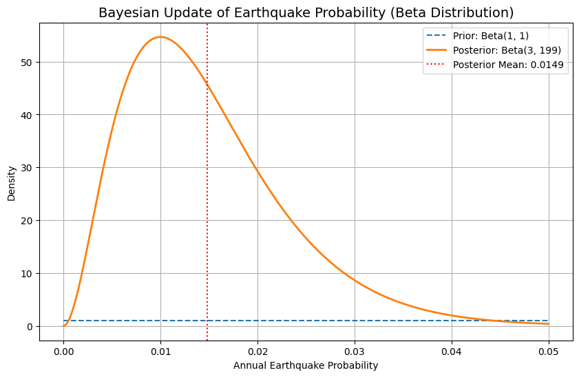
Output Summary:
- Posterior Mean: ~0.01485, or 1.48% annual probability
- You’ll see how the belief about the earthquake probability shifts from a uniform prior to a sharper peak after observing two events in 200 years.
Let me know if you want to simulate further updates (e.g., new earthquake in year 201), or integrate this into a web app or dashboard.