We’re often told that the R² value in a regression model ranges between 0 and 1. A score close to 1? Great model! A score near 0? Not so great.
But here’s a question most textbooks skip:
Can R² be negative?
Yes. And when it is, it’s a big red flag.
Let me walk you through why — with code, plots, and a surprising mathematical twist.
When Guessing Outperforms Your Model
Imagine you’re trying to predict house prices.
But instead of using real-world features like square footage or number of rooms…
You train your model using just the row index of the dataset (0, 1, 2, …).
You know it won’t perform well — but how badly?
Let’s find out:
import numpy as np
from sklearn.linear_model import LinearRegression
from sklearn.metrics import r2_score
import matplotlib.pyplot as plt

# Actual data: decreasing trend
X = np.array([[1], [2], [3], [4], [5]])
y = np.array([10, 8, 6, 4, 2])

# Bad model: predict constant (wrong!) values
y_bad = np.array([5, 5, 5, 5, 5])
model = LinearRegression()
model.fit(X, y_bad)  # Fitting on wrong y

# Predict on true y values
y_pred = model.predict(X)
r2 = r2_score(y, y_pred)

# Output R²
print("R² Score:", r2)

# Plot
plt.scatter(X, y, color='blue', label='Actual data')
plt.plot(X, y_pred, color='red', label='Bad model')
plt.axhline(np.mean(y), color='green', linestyle='--', label='Mean of y')
plt.title(f"Bad Model Fit (R² = {r2:.2f})")
plt.legend()
plt.grid(True)
plt.show()
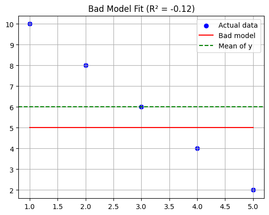
The model is worse than predicting the average, which gives you a negative R². That’s not a bug — that’s your model admitting defeat.
So :
- R² is not a square in the arithmetic sense.
- Squaring a number like
 is different — even complex numbers behave differently.
 - But R² is about how well your model captures variability. And if it performs poorly, R² will let you know — even with a minus sign.
Bottom line:
If you get a negative R², it’s your model’s polite way of saying:
“You’d be better off guessing the mean.”
What Does Negative R² Really Mean?
Mathematically, R² is defined as:
textCopyEditR² = 1 - (SS_res / SS_tot)
- SS_res: residual sum of squares (errors of the model)
- SS_tot: total sum of squares (errors of the mean-only model)
If your model’s error is larger than that of a “dumb” average-based prediction,
then SS_res > SS_tot → R² becomes negative.
So, in plain English:
A negative R² means your model performs worse than no model at all.
Let’s Clear Up a Common Misconception: “Squared” Doesn’t Mean Power
The name R-squared misleads many into thinking it’s always non-negative — like squaring a number.
But here’s the catch:
- The “squared” in R² comes from squaring residuals (the errors),
not from squaring some kind of correlation coefficient. - It’s a statistical measure, not a mathematical power operation.
In fact, real squaring behaves differently:
x = 3
print(x**2)  # 9
print((-3)**2)  # 9
Always positive.
But when you move into complex numbers, things get spicier:
import cmath
z = complex(0, 1)  # i
print(z**2)  # Output: (-1+0j)
Yes — i² = -1.
So, squaring in complex math can result in negative values.
Key Takeaways for Readers
- R² < 0 means your model is worse than guessing.
Always check your features and assumptions. - “Squared” in R² doesn’t mean it behaves like math powers.
It’s a statistical ratio, not a square root or power-of-two operation. - In complex numbers, squared values can be negative — just like R².
That’s a fun coincidence, not a cause — but it’s a helpful analogy. - Always use R² with other metrics: residual plots, p-values, and domain intuition.


 is the average rate of occurrence. For example, it can model the number of earthquakes per century.
 and
and  represent the location, scale, and shape of the distribution respectively. EVT is widely used in engineering, hydrology, and seismology.

 :
:


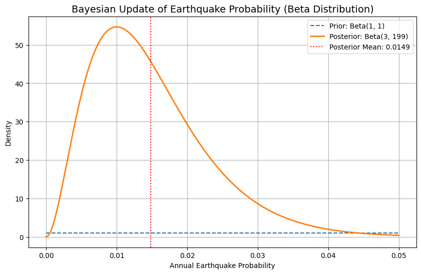
![$$ E[\theta]=\frac{3}{3+199}=\frac{3}{202} \approx 0.0148 $$](https://codetipsacademy.com/wp-content/ql-cache/quicklatex.com-be5c5b6a67d5e1b9e2d958888115c613_l3.png "Rendered by QuickLaTeX.com")


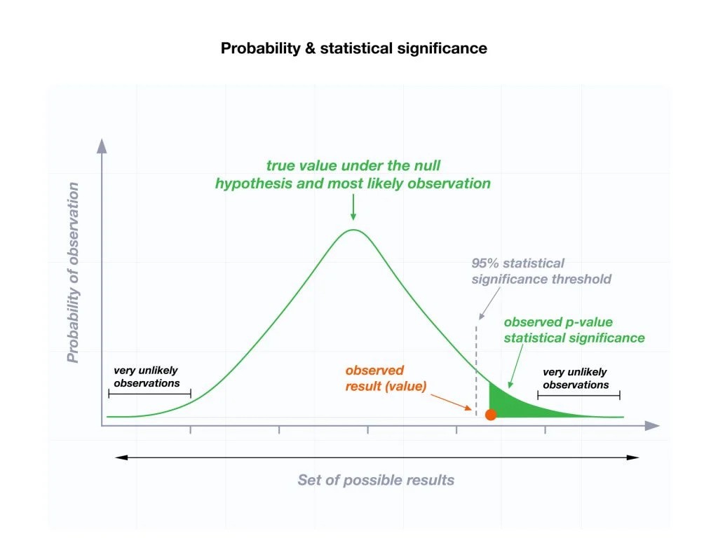
 (or more extreme) under the assumption that the null hypothesis
  is true.